Connecting the Dots – Supervised Learning
We can connect this to vectors and matrices. Let’s dig into it and see how everything fits together.
Statement:
“If we only use y = m * x, our line always goes through (0,0)”
That is true in both:
- Basic algebra (2D lines)
- Linear algebra (vectors/matrices)
And yes — this behavior is deeply rooted in how matrix multiplication works.
In Simple Algebra:
A line like:
y=m∗x
means:
When x = 0, y = 0 — always.
So the line must go through the origin (0, 0).
We can’t move the line up or down without adding a bias (intercept) like this:
y=m∗x+c
In Linear Algebra (Vectors and Matrices):
When using matrix multiplication for linear models:
y = X @ W
- X is our input matrix (shape: [n_samples, n_features])
- W is our weights vector (shape: [n_features, 1])
- y is the output (predicted values)
This is a pure linear transformation.
And here’s the rule:
Linear transformations always map the origin (0) to the origin.
So if our model is:
y=X@W
Then:
If X=[0],y=0
That’s the same as forcing the line to pass through (0,0).
To Shift the Line (or Plane), an Affine Transformation needed
That’s where we add bias (b):
y=X@W+b
This is now an affine transformation — linear + shift.
It lets our model move the line (or decision boundary) up/down/around to better match the data.
Summary Table:
| Equation | Type | Goes through origin? | Can shift? |
|---|---|---|---|
| y = m * x | Linear | Yes | No |
| y = m * x + c | Affine (shifted line) | Not always | Yes |
| y = X @ W | Linear (matrix) | Yes | No |
| y = X @ W + b | Affine (matrix) | Not always | Yes |
Final Answer:
The reason y = m * x (or y = X @ W) always passes through the origin is a fundamental property of linear transformations in vector/matrix algebra.
Adding + c or + b makes it affine, not purely linear — and allows the model to learn any offset, not just the slope.
Let’s build a NumPy demo that shows the difference between:
A pure linear transformation (y = W * x)
An affine transformation (y = W * x + b)
We’ll visualize both so we can see how the bias shifts the line.
Python Code with Plot (Linear vs. Affine)
import numpy as np
import matplotlib.pyplot as plt
# Inputs (x values)
X = np.array([[0], [1], [2], [3], [4], [5]])
# Target equation: y = 2x + 1
W = np.array([2]) # weight/slope
b = np.array([1]) # bias/intercept
# Pure Linear Transformation (no bias): y = W * x
y_linear = X @ W # Same as np.dot(X, W), no intercept
# Affine Transformation (with bias): y = W * x + b
y_affine = X @ W + b
# Plot both
plt.figure(figsize=(8, 5))
plt.plot(X, y_linear, label="Linear: y = 2x", linestyle='--', color='blue')
plt.plot(X, y_affine, label="Affine: y = 2x + 1", linestyle='-', color='green')
plt.scatter(X, y_affine, color='green')
plt.axhline(0, color='gray', linewidth=0.5)
plt.axvline(0, color='gray', linewidth=0.5)
# Labels and legend
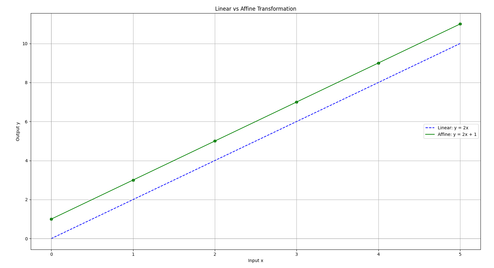
plt.title("Linear vs Affine Transformation")
plt.xlabel("Input x")
plt.ylabel("Output y")
plt.legend()
plt.grid(True)
plt.show()
What we’ll See:
- Dashed Blue Line (y = 2x): always passes through (0,0)
- Solid Green Line (y = 2x + 1): same slope, but shifted up by 1
Summary:
y = W * x is a pure linear transformation → can only rotate/scale, no shift.
y = W * x + b is an affine transformation → can rotate/scale and shift.
This is why machine learning models almost always include a bias term — it gives them the flexibility to fit more real-world data.
Supervised Learning – Summary