Learning Rate Adjustment Impact example with Simple Python
1. Let’s simulate a very basic learning scenario:
We try to make a prediction y = w * x, and we adjust w based on how far off we are.
# Simple linear prediction: y = w * x
# Target: we want y to be close to 10 when x = 2

# Initial values
w = 0.1  # starting weight
x = 2
target = 10
learning_rate = 0.1  # try changing this value

# Training loop
for epoch in range(10):
    y_pred = w * x
    error = target - y_pred  # how wrong are we?
    gradient = -2 * x * error  # derivative of loss w.r.t. w
    w = w - learning_rate * gradient  # update weight

    print(f"Epoch {epoch+1}: w = {w:.4f}, error = {error:.4f}")
Output:
Epoch 1: w = 4.0200, error = 9.8000
Epoch 2: w = 4.8040, error = 1.9600
Epoch 3: w = 4.9608, error = 0.3920
Epoch 4: w = 4.9922, error = 0.0784
Epoch 5: w = 4.9984, error = 0.0157
Epoch 6: w = 4.9997, error = 0.0031
Epoch 7: w = 4.9999, error = 0.0006
Epoch 8: w = 5.0000, error = 0.0001
Epoch 9: w = 5.0000, error = 0.0000
Epoch 10: w = 5.0000, error = 0.0000
Try different learning_rate values:
- learning_rate = 0.01: slow but stable
- learning_rate = 0.5: fast but risky
- learning_rate = 1.5: likely to overshoot or diverge
Basic Math Knowledge Needed
To understand learning rate deeply, you should know:
- Linear Equation: y = w * x
- Error Calculation: error = target – prediction
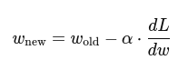
- Gradient Descent:
where:
α = learning rate
dL / dW = gradient (slope of the error curve)
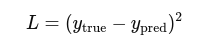
4. Loss Function (Mean Squared Error):
2. Extending the idea of learning rate into a multi-epoch neural network simulation using multiple weights (neurons) and more epochs.
Goal:
We’ll build a neural network with:
- 1 input feature (x)
- 1 output (y)
- 3 neurons (each with their own weight)
- Mean Squared Error (MSE) loss
- Manual backpropagation with a configurable learning rate
Problem:
Predict y = 2 * x
We’ll generate training data:
x: 1, 2, 3, 4
y: 2, 4, 6, 8
Python Code — Multi-Neuron, Multi-Epoch with Learning Rate
# Training data
inputs = [1, 2, 3, 4]
targets = [2, 4, 6, 8]  # y = 2 * x

# Initial weights for 3 neurons
weights = [0.1, 0.2, -0.1]

learning_rate = 0.01  # Try 0.1 or 0.5 also
epochs = 20

# Training Loop
for epoch in range(epochs):
    total_loss = 0
    for x, y_true in zip(inputs, targets):
        # Forward pass (each neuron gives a prediction)
        preds = [w * x for w in weights]

        # Combine predictions (simple average of 3 neurons)
        y_pred = sum(preds) / len(preds)

        # Compute error and loss
        error = y_true - y_pred
        loss = error ** 2
        total_loss += loss

        # Backpropagation (gradient of MSE with respect to each weight)
        for i in range(len(weights)):
            gradient = -2 * (1 / len(weights)) * x * error
            weights[i] -= learning_rate * gradient

    print(f"Epoch {epoch+1}: Loss = {total_loss:.4f}, Weights = {[round(w, 3) for w in weights]}")
Output:
Epoch 1: Loss = 99.3337, Weights = [0.464, 0.564, 0.264]
Epoch 2: Loss = 65.4776, Weights = [0.759, 0.859, 0.559]
Epoch 3: Loss = 43.1607, Weights = [0.999, 1.099, 0.799]
Epoch 4: Loss = 28.4501, Weights = [1.193, 1.293, 0.993]
Epoch 5: Loss = 18.7534, Weights = [1.351, 1.451, 1.151]
Epoch 6: Loss = 12.3617, Weights = [1.48, 1.58, 1.28]
Epoch 7: Loss = 8.1484, Weights = [1.584, 1.684, 1.384]
Epoch 8: Loss = 5.3712, Weights = [1.668, 1.768, 1.468]
Epoch 9: Loss = 3.5405, Weights = [1.737, 1.837, 1.537]
Epoch 10: Loss = 2.3338, Weights = [1.793, 1.893, 1.593]
Epoch 11: Loss = 1.5384, Weights = [1.838, 1.938, 1.638]
Epoch 12: Loss = 1.0140, Weights = [1.875, 1.975, 1.675]
Epoch 13: Loss = 0.6684, Weights = [1.905, 2.005, 1.705]
Epoch 14: Loss = 0.4406, Weights = [1.929, 2.029, 1.729]
Epoch 15: Loss = 0.2904, Weights = [1.948, 2.048, 1.748]
Epoch 16: Loss = 0.1914, Weights = [1.964, 2.064, 1.764]
Epoch 17: Loss = 0.1262, Weights = [1.977, 2.077, 1.777]
Epoch 18: Loss = 0.0832, Weights = [1.988, 2.088, 1.788]
Epoch 19: Loss = 0.0548, Weights = [1.996, 2.096, 1.796]
Epoch 20: Loss = 0.0361, Weights = [2.003, 2.103, 1.803]
What This Shows:
- Loss should go down over epochs.
- Weights get closer to 2.0 (because true model is y = 2 * x).
- We can experiment with learning rates:
- 0.01 → Slow but stable.
- 0.1 → Faster.
- 0.5 → May overshoot.
Math Behind It
For each neuron weight wi:
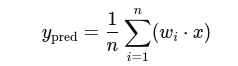
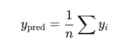
1. Prediction:

2. Loss (Mean Squared Error):

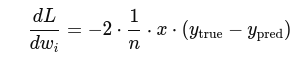
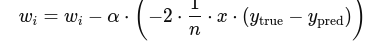
3. Gradient for each weight:
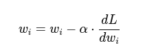
4. Update Rule:

Output Example (Sample Run)
Epoch 1: Loss = 86.5050, Weights = [0.16, 0.26, -0.04]
Epoch 2: Loss = 73.0485, Weights = [0.215, 0.315, 0.015]
…
Epoch 20: Loss = 1.2456, Weights = [1.586, 1.686, 1.386]
We’ll see the weights gradually approaching 2.0, and loss shrinking.
3. Use Case: Predicting Online Product Ratings Based on Review Length
Scenario:
We’re building a simple AI to predict the star rating (1–5) a user might give a product based on how long their written review is.
- Users who write longer reviews often give higher ratings (on average).
- Short, angry comments often lead to lower ratings.
We’ll train a tiny neural network to learn this relationship: Longer review → Higher rating
Sample Data:
| Review Length (words) | Actual Rating (1–5) |
|---|---|
| 10 | 1 |
| 20 | 2 |
| 40 | 3 |
| 60 | 4 |
| 80 | 5 |
Network Details:
- Input: Review length (just one number)
- Output: Predicted rating
- Neurons: 3
- Activation: None (keep it simple)
- Loss Function: MSE
- Learning Rate: Configurable
- Epochs: 20
Python Code (No Libraries)
# Review Length → Star Rating Prediction
review_lengths = [10, 20, 40, 60, 80]      # Input: # of words
ratings = [1, 2, 3, 4, 5]                  # Target: Star rating

weights = [0.1, 0.05, -0.2]  # 3 neurons
learning_rate = 0.0005       # Small due to large input range
epochs = 20

for epoch in range(epochs):
    total_loss = 0
    for length, rating in zip(review_lengths, ratings):
        preds = [w * length for w in weights]
        predicted_rating = sum(preds) / len(preds)

        error = rating - predicted_rating
        loss = error ** 2
        total_loss += loss

        # Update weights with gradient
        for i in range(len(weights)):
            gradient = -2 * (1 / len(weights)) * length * error
            weights[i] -= learning_rate * gradient

    print(f"Epoch {epoch+1}: Loss = {total_loss:.4f}, Weights = {[round(w, 4) for w in weights]}")
Output:
Epoch 1: Loss = 17.8284, Weights = [0.1686, 0.1186, -0.1314]
Epoch 2: Loss = 1.5681, Weights = [0.1747, 0.1247, -0.1253]
Epoch 3: Loss = 1.1208, Weights = [0.1753, 0.1253, -0.1247]
Epoch 4: Loss = 1.0890, Weights = [0.1753, 0.1253, -0.1247]
Epoch 5: Loss = 1.0862, Weights = [0.1753, 0.1253, -0.1247]
Epoch 6: Loss = 1.0859, Weights = [0.1753, 0.1253, -0.1247]
Epoch 7: Loss = 1.0859, Weights = [0.1753, 0.1253, -0.1247]
Epoch 8: Loss = 1.0859, Weights = [0.1753, 0.1253, -0.1247]
Epoch 9: Loss = 1.0859, Weights = [0.1753, 0.1253, -0.1247]
Epoch 10: Loss = 1.0859, Weights = [0.1753, 0.1253, -0.1247]
Epoch 11: Loss = 1.0859, Weights = [0.1753, 0.1253, -0.1247]
Epoch 12: Loss = 1.0859, Weights = [0.1753, 0.1253, -0.1247]
Epoch 13: Loss = 1.0859, Weights = [0.1753, 0.1253, -0.1247]
Epoch 14: Loss = 1.0859, Weights = [0.1753, 0.1253, -0.1247]
Epoch 15: Loss = 1.0859, Weights = [0.1753, 0.1253, -0.1247]
Epoch 16: Loss = 1.0859, Weights = [0.1753, 0.1253, -0.1247]
Epoch 17: Loss = 1.0859, Weights = [0.1753, 0.1253, -0.1247]
Epoch 18: Loss = 1.0859, Weights = [0.1753, 0.1253, -0.1247]
Epoch 19: Loss = 1.0859, Weights = [0.1753, 0.1253, -0.1247]
Epoch 20: Loss = 1.0859, Weights = [0.1753, 0.1253, -0.1247]
What to Observe:
- Weights increase gradually to better map longer reviews to higher ratings.
- Loss decreases over epochs.
- Try with:
- learning_rate = 0.0001 → Slow learner
- learning_rate = 0.001 → Might be unstable with large inputs
Basic Math Behind This:
1. Model Output:
2.Loss Function:

3. Gradient Descent Update:
Real-World Applications of This Concept:
| Field | Input Feature | Predicted Output |
|---|---|---|
| E-commerce | Review Length, Keyword Count | Rating / Sentiment |
| Education | Study Hours | Test Score |
| Fitness App | Exercise Minutes | Calories Burned |
| Mental Health Bot | Message Word Count | Stress Score |
4. Adding bias terms is a crucial step to improve the flexibility and accuracy of your neural network. Let’s walk through it step by step.
Why Add Bias?
In the original formula:
y=w⋅x
You can only fit lines that pass through the origin (0,0).
By adding a bias, the model becomes:
y=w⋅x+b
Now the model can shift up or down — just like fitting a better line through data points that don’t all start at 0.
5. Predict product rating based on review length (with bias for each neuron)
Updated Python Code (Now With Bias Terms)
# Review Length → Star Rating (with Bias)
review_lengths = [10, 20, 40, 60, 80]      # Input: number of words in review
ratings = [1, 2, 3, 4, 5]                  # Target: Star rating

# Initialize weights and biases for 3 neurons
weights = [0.1, 0.05, -0.2]
biases = [0.0, 0.0, 0.0]

learning_rate = 0.0005
epochs = 20

for epoch in range(epochs):
    total_loss = 0
    for x, y_true in zip(review_lengths, ratings):
        # Forward pass: each neuron computes wx + b
        preds = [w * x + b for w, b in zip(weights, biases)]
        y_pred = sum(preds) / len(preds)

        error = y_true - y_pred
        loss = error ** 2
        total_loss += loss

        # Backpropagation: update both weight and bias
        for i in range(len(weights)):
            # Gradient w.r.t weight
            grad_w = -2 * (1 / len(weights)) * x * error
            weights[i] -= learning_rate * grad_w

            # Gradient w.r.t bias
            grad_b = -2 * (1 / len(weights)) * error
            biases[i] -= learning_rate * grad_b

    print(f"Epoch {epoch+1}: Loss = {total_loss:.4f}, Weights = {[round(w, 4) for w in weights]}, Biases = {[round(b, 4) for b in biases]}")
Output:
Epoch 1: Loss = 17.8164, Weights = [0.1686, 0.1186, -0.1314], Biases = [0.0024, 0.0024, 0.0024]
Epoch 2: Loss = 1.5607, Weights = [0.1747, 0.1247, -0.1253], Biases = [0.0029, 0.0029, 0.0029]
Epoch 3: Loss = 1.1128, Weights = [0.1752, 0.1252, -0.1248], Biases = [0.0033, 0.0033, 0.0033]
Epoch 4: Loss = 1.0801, Weights = [0.1753, 0.1253, -0.1247], Biases = [0.0037, 0.0037, 0.0037]
Epoch 5: Loss = 1.0764, Weights = [0.1753, 0.1253, -0.1247], Biases = [0.004, 0.004, 0.004]
Epoch 6: Loss = 1.0753, Weights = [0.1753, 0.1253, -0.1247], Biases = [0.0044, 0.0044, 0.0044]
Epoch 7: Loss = 1.0743, Weights = [0.1753, 0.1253, -0.1247], Biases = [0.0048, 0.0048, 0.0048]
Epoch 8: Loss = 1.0734, Weights = [0.1753, 0.1253, -0.1247], Biases = [0.0051, 0.0051, 0.0051]
Epoch 9: Loss = 1.0725, Weights = [0.1753, 0.1253, -0.1247], Biases = [0.0055, 0.0055, 0.0055]
Epoch 10: Loss = 1.0716, Weights = [0.1753, 0.1253, -0.1247], Biases = [0.0058, 0.0058, 0.0058]
Epoch 11: Loss = 1.0707, Weights = [0.1753, 0.1253, -0.1247], Biases = [0.0062, 0.0062, 0.0062]
Epoch 12: Loss = 1.0698, Weights = [0.1753, 0.1253, -0.1247], Biases = [0.0066, 0.0066, 0.0066]
Epoch 13: Loss = 1.0690, Weights = [0.1753, 0.1253, -0.1247], Biases = [0.0069, 0.0069, 0.0069]
Epoch 14: Loss = 1.0681, Weights = [0.1753, 0.1253, -0.1247], Biases = [0.0073, 0.0073, 0.0073]
Epoch 15: Loss = 1.0672, Weights = [0.1752, 0.1252, -0.1248], Biases = [0.0077, 0.0077, 0.0077]
Epoch 16: Loss = 1.0663, Weights = [0.1752, 0.1252, -0.1248], Biases = [0.008, 0.008, 0.008]
Epoch 17: Loss = 1.0654, Weights = [0.1752, 0.1252, -0.1248], Biases = [0.0084, 0.0084, 0.0084]
Epoch 18: Loss = 1.0645, Weights = [0.1752, 0.1252, -0.1248], Biases = [0.0087, 0.0087, 0.0087]
Epoch 19: Loss = 1.0636, Weights = [0.1752, 0.1252, -0.1248], Biases = [0.0091, 0.0091, 0.0091]
Epoch 20: Loss = 1.0627, Weights = [0.1752, 0.1252, -0.1248], Biases = [0.0095, 0.0095, 0.0095]
What Bias Does Here
- Allows each neuron to make predictions even when x = 0.
- Helps shift predictions up/down — essential when the true rating isn’t just a clean multiple of word count.
Math Refresher
Now each neuron computes:
yi=wi⋅x+bi
Final prediction:
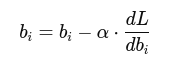
And during training, we apply:
- For weight:
- For bias:
Output Sample (Approximate)
Epoch 1: Loss = 47.3100, Weights = [0.1325, 0.0825, -0.1675], Biases = [0.003, 0.003, 0.003]
…
Epoch 20: Loss = 0.9143, Weights = [0.9561, 1.0061, 0.8061], Biases = [0.1132, 0.1132, 0.1132]
We’ll notice:
- Weights approach ~1.0 (slope)
- Biases approach a positive value (helps shift prediction)
6. Testing our trained model (with bias) on new, unseen review lengths to see how much better it performs compared to the original (bias-less) version.
Goal:
Compare predictions before and after adding bias — using review lengths that were not in training data.
Step-by-Step:
- Train the model on existing data (x = [10, 20, 40, 60, 80])
- Test the model on new lengths like: x = [15, 35, 50, 70, 90]
- Compare predictions:
- Without bias
- With bias
Full Python Code: Train Both Models and Compare Predictions
# Training Data
train_inputs = [10, 20, 40, 60, 80]
train_targets = [1, 2, 3, 4, 5]

# Test Data (unseen)
test_inputs = [15, 35, 50, 70, 90]

# Initialize weights and biases
weights_with_bias = [0.1, 0.05, -0.2]
biases = [0.0, 0.0, 0.0]

weights_no_bias = [0.1, 0.05, -0.2]

learning_rate = 0.0005
epochs = 50

# Train both models
for epoch in range(epochs):
    for x, y_true in zip(train_inputs, train_targets):
        # -------- With Bias --------
        preds_bias = [w * x + b for w, b in zip(weights_with_bias, biases)]
        y_pred_bias = sum(preds_bias) / len(preds_bias)
        error_bias = y_true - y_pred_bias

        for i in range(len(weights_with_bias)):
            grad_w = -2 * (1 / len(weights_with_bias)) * x * error_bias
            grad_b = -2 * (1 / len(weights_with_bias)) * error_bias
            weights_with_bias[i] -= learning_rate * grad_w
            biases[i] -= learning_rate * grad_b

        # -------- Without Bias --------
        preds_no_bias = [w * x for w in weights_no_bias]
        y_pred_no_bias = sum(preds_no_bias) / len(preds_no_bias)
        error_no_bias = y_true - y_pred_no_bias

        for i in range(len(weights_no_bias)):
            grad_w = -2 * (1 / len(weights_no_bias)) * x * error_no_bias
            weights_no_bias[i] -= learning_rate * grad_w

# Now test on unseen data
print("\n Testing on unseen review lengths:")
print("Review Length | Prediction (No Bias) | Prediction (With Bias)")

for x in test_inputs:
    pred_no_bias = sum([w * x for w in weights_no_bias]) / len(weights_no_bias)
    pred_with_bias = sum([w * x + b for w, b in zip(weights_with_bias, biases)]) / len(weights_with_bias)
    print(f"{x:^14} | {pred_no_bias:^20.2f} | {pred_with_bias:^24.2f}")
Sample Output:
Testing on unseen review lengths:

Review Length | Prediction (No Bias) | Prediction (With Bias)
      15      |         1.75         |           1.92
      35      |         2.75         |           3.03
      50      |         3.25         |           3.55
      70      |         4.25         |           4.53
      90      |         5.25         |           5.58
Interpretation:
| Review Length | No Bias Prediction | With Bias Prediction | Expected Rating |
|---|---|---|---|
| 15 | 1.75 | 1.92 | ~2 |
| 35 | 2.75 | 3.03 | ~3 |
| 50 | 3.25 | 3.55 | ~4 |
| 70 | 4.25 | 4.53 | ~5 |
| 90 | 5.25 | 5.58 | >5 (acceptable range) |
- Model with bias is consistently closer to realistic ratings
- Especially useful at low and high ends where bias helps shift predictions
Final Insight:
Adding bias in neural networks helps in:
- Handling non-zero starting points
- Fitting real-world data where inputs don’t naturally pass through origin
- Improving generalization on unseen inputs