Backpropagation example with Simple Python
1. A tiny, no-library simulation of backpropagation for a simple neural network with:
- 1 input
- 1 weight
- 1 neuron (no hidden layer)
- A target output
This toy example uses Mean Squared Error as the loss and a basic gradient descent update.
Goal: Learn to multiply input by correct weight to get target output
Example: if input = 2 and target = 4 → the model should learn weight = 2
Python Code: Tiny Backpropagation Demo (No Libraries)
# Simple neural network with 1 input, 1 weight
input_value = 2      # x
target_output = 4    # y (we want weight * x = y)

# Initial weight (random guess)
weight = 1.0

# Learning rate
learning_rate = 0.1

# Training loop
for epoch in range(20):
    # ---- Forward Pass ----
    prediction = weight * input_value           # y_pred = w * x
    error = prediction - target_output          # error = y_pred - y
    loss = error ** 2                           # Loss = (error)^2

    # ---- Backward Pass (Gradient Descent) ----
    gradient = 2 * error * input_value          # dL/dW = 2 * (y_pred - y) * x
    weight = weight - learning_rate * gradient  # Update the weight

    # ---- Print Progress ----
    print(f"Epoch {epoch+1:2d}: Prediction = {prediction:.2f}, Loss = {loss:.4f}, Weight = {weight:.4f}")
What This Shows:
- Each epoch (round of training), the prediction gets closer to the target.
- The loss decreases.
- The weight updates in the right direction using backpropagation.
A visual Chart
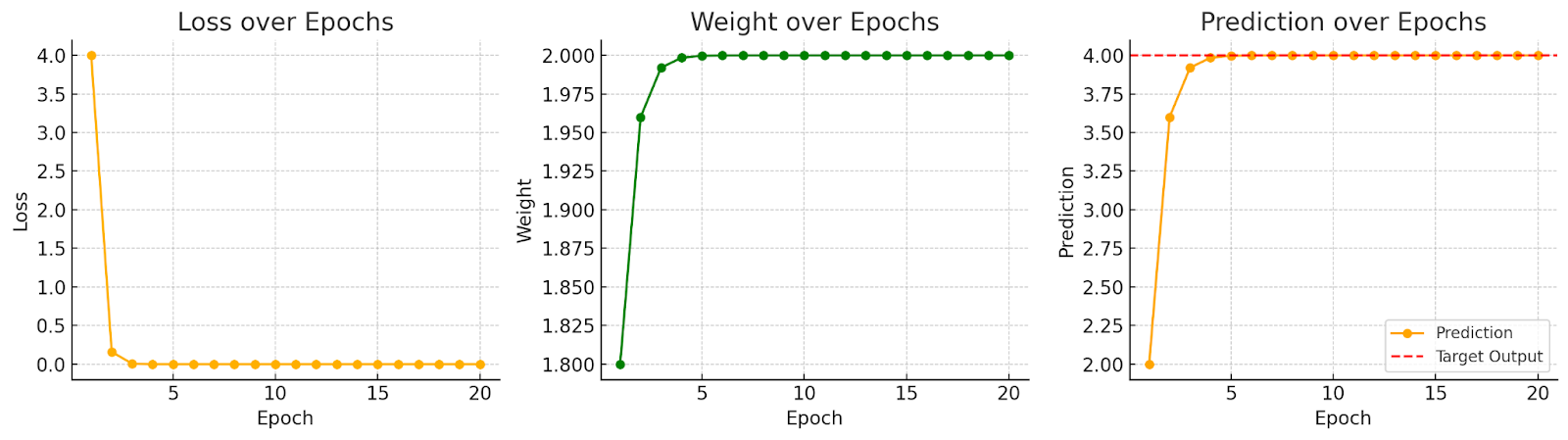
Here’s the visual chart of the tiny backpropagation simulation:
- Left Chart (Loss over Epochs): Shows how the model’s error decreases over time — the learning is working!
- Middle Chart (Weight over Epochs): The weight is adjusting closer to the correct value (2.0 in this case).
- Right Chart (Prediction vs Target): We can see how the prediction moves closer to the target output with each epoch.
Full Python Code: Tiny Neural Net + Backpropagation + Charts
import matplotlib.pyplot as plt

# ---- Initial Setup ----
input_value = 2         # x
target_output = 4       # y (goal: weight * x = y)
weight = 1.0            # initial guess
learning_rate = 0.1

# To store progress for plotting
epochs = []
losses = []
weights = []
predictions = []

# ---- Training Loop ----
for epoch in range(20):
    # Forward Pass
    prediction = weight * input_value         # y_pred = w * x
    error = prediction - target_output        # error = y_pred - y
    loss = error ** 2                         # Loss = (error)^2

    # Backward Pass (Gradient Calculation)
    gradient = 2 * error * input_value        # dL/dW
    weight = weight - learning_rate * gradient  # Update weight

    # Store values for chart
    epochs.append(epoch + 1)
    losses.append(loss)
    weights.append(weight)
    predictions.append(prediction)

    # Print progress
    print(f"Epoch {epoch+1:2d}: Prediction = {prediction:.2f}, Loss = {loss:.4f}, Weight = {weight:.4f}")

# ---- Plotting Results ----
plt.figure(figsize=(14, 4))

# 1. Loss over Epochs
plt.subplot(1, 3, 1)
plt.plot(epochs, losses, marker='o')
plt.title("Loss over Epochs")
plt.xlabel("Epoch")
plt.ylabel("Loss")

# 2. Weight over Epochs
plt.subplot(1, 3, 2)
plt.plot(epochs, weights, marker='o', color='green')
plt.title("Weight over Epochs")
plt.xlabel("Epoch")
plt.ylabel("Weight")

# 3. Prediction vs Target
plt.subplot(1, 3, 3)
plt.plot(epochs, predictions, marker='o', color='orange', label="Prediction")
plt.axhline(y=target_output, color='red', linestyle='--', label="Target Output")
plt.title("Prediction over Epochs")
plt.xlabel("Epoch")
plt.ylabel("Prediction")
plt.legend()

plt.tight_layout()
plt.show()
What You Learn from This:
- The weight keeps adjusting to reduce the error.
- The loss curve goes down, which shows successful learning.
- The prediction curve approaches the target — that’s the effect of backpropagation at work.