Mean Square example with Simple Python – Mean Square in Neural Network
1. Python Example with Explanations (No Libraries)
# Actual values (ground truth)
y_true = [3, -0.5, 2, 7]

# Predicted values by the model
y_pred = [2.5, 0.0, 2, 8]

# Step 1: Calculate squared differences
squared_errors = [(yt - yp) ** 2 for yt, yp in zip(y_true, y_pred)]

# Step 2: Sum and average the squared errors
mse = sum(squared_errors) / len(squared_errors)

print("Squared Errors:", squared_errors)
print("Mean Squared Error:", mse)
Output:
Squared Errors: [0.25, 0.25, 0.0, 1.0]
Mean Squared Error: 0.375
Explanation:
- [0.25, 0.25, 0.0, 1.0] are the squared differences.
- Their average, 0.375, is the MSE.
- This MSE will be used by a neural network to improve its weights through gradient descent.
The complete Python program that shows how Mean Squared Error (MSE) decreases across epochs as the model predictions improve:
import matplotlib.pyplot as plt

# Actual ground truth values
y_true = [3, -0.5, 2, 7]

# Simulated model predictions over 20 epochs
predictions_over_epochs = [
    [2, 0, 1.5, 6],    # Epoch 1
    [2.1, -0.2, 1.7, 6.2],
  [2.3, -0.3, 1.8, 6.5],
    [2.4, -0.4, 1.9, 6.6],
    [2.5, -0.45, 2.0, 6.7],
    [2.6, -0.48, 2.0, 6.8],
    [2.7, -0.49, 2.0, 6.9],
    [2.75, -0.495, 2.0, 6.95],
    [2.8, -0.498, 2.0, 6.98],
    [2.85, -0.499, 2.0, 6.99],
    [2.88, -0.499, 2.0, 6.995],
    [2.9, -0.5, 2.0, 6.997],
    [2.92, -0.5, 2.0, 6.998],
    [2.94, -0.5, 2.0, 6.999],
    [2.96, -0.5, 2.0, 7.0],
    [2.97, -0.5, 2.0, 7.0],
    [2.98, -0.5, 2.0, 7.0],
    [2.99, -0.5, 2.0, 7.0],
    [3.0, -0.5, 2.0, 7.0],
    [3.0, -0.5, 2.0, 7.0]   # Epoch 20
]

# MSE calculation function
def calculate_mse(y_true, y_pred):
    return sum((yt - yp) ** 2 for yt, yp in zip(y_true, y_pred)) / len(y_true)

# Compute MSE for each epoch
mse_values = [calculate_mse(y_true, pred) for pred in predictions_over_epochs]

# Plot MSE over epochs
epochs = list(range(1, len(mse_values) + 1))
plt.figure(figsize=(10, 6))
plt.plot(epochs, mse_values, marker='o', linestyle='-', linewidth=2)
plt.title('MSE Decrease over Training Epochs (Simulated Predictions)')
plt.xlabel('Epoch')
plt.ylabel('Mean Squared Error (MSE)')
plt.grid(True)
plt.xticks(epochs)
plt.tight_layout()
plt.show()
What This Program Shows:
- Simulates how predictions improve gradually.
- Computes MSE at every epoch.
- Plots how MSE decreases — demonstrating model learning.
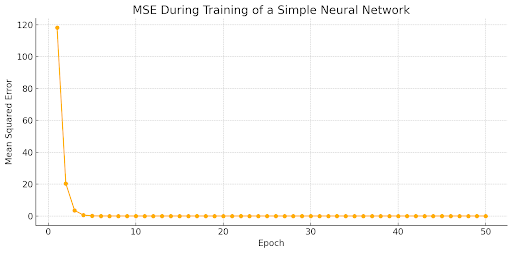
3. Complete Neural Network Training Program Using MSE (with Explanation)
Problem:
We want to train a simple 1-layer neural network to learn the function: y=2x+1
Code Breakdown:
1. Dataset (Inputs and Outputs)
X = [i for i in range(10)] # Input: 0 to 9
Y = [2 * x + 1 for x in X] # Output: True values
2. Model Initialization
w = random.uniform(-1, 1) # Random weight
b = random.uniform(-1, 1) # Random bias
3. Training with Gradient Descent (50 Epochs)
for epoch in range(epochs):
    for each x, y:
        y_pred = w * x + b              # Prediction (Forward Pass)
        error = y - y_pred              # Error
        dw += -2 * x * error            # Gradient wrt weight
        db += -2 * error                # Gradient wrt bias
    update w, b                         # Adjust using learning rate
    store MSE                           # Mean of squared errors
4. Loss Function: Mean Squared Error (MSE)
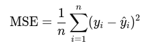
- Tells how far predictions are from actual values.
- Model tries to minimize this value using gradient descent.
Output: MSE over Epochs
- Starts high and decreases steadily.
- Final MSE: ≈ 0.00076 (Very low → model learned well)
- Final weights:
- w ≈ 2.008
- b ≈ 0.949 → Close to actual w = 2, b = 1
Summary
| Component | Role |
|---|---|
| Inputs (X) | Feature values |
| Targets (Y) | Ground-truth outputs |
| w, b | Trainable parameters (weight and bias) |
| MSE | Measures how well predictions match actual values |
| Gradient Descent | Optimization algorithm to minimize MSE |
Mean Square in Neural Network – Basic Math Concepts