Kernel In Regression example with Simple Python
Story-Like Explanation – “The Farmer and the Curvy Field”
1. Goal
We’ll simulate a non-linear function, like: y=sin(2πx)+noisey
And then fit it using RBF kernel regression (Kernel Ridge Regression).
Required Libraries
import numpy as np
import matplotlib.pyplot as plt
from sklearn.kernel_ridge import KernelRidge
Step-by-Step Implementation
# Step 1: Generate Sample Nonlinear Data
np.random.seed(42)
X = np.linspace(0, 1, 50).reshape(-1, 1)
y = np.sin(2 * np.pi * X).ravel() + np.random.normal(0, 0.1, X.shape[0])

# Step 2: Fit Kernel Ridge Regression with RBF Kernel
model = KernelRidge(kernel='rbf', alpha=1.0, gamma=15)
model.fit(X, y)

# Step 3: Predict on a fine grid for smooth curve
X_test = np.linspace(0, 1, 500).reshape(-1, 1)
y_pred = model.predict(X_test)

# Step 4: Plot Results
plt.figure(figsize=(10, 5))
plt.scatter(X, y, color='red', label='Training data')
plt.plot(X_test, y_pred, color='blue', label='RBF Kernel Regression')
plt.title('Kernel Regression using RBF Kernel')
plt.xlabel('x')
plt.ylabel('y')
plt.legend()
plt.grid(True)
plt.show()
Explanation of Parameters
| Parameter | Description |
|---|---|
| alpha | Regularization term (like λ in ridge regression) |
| kernel=’rbf’ | Radial Basis Function kernel |
| gamma | Controls the width of the RBF kernel: higher = narrow bumps, lower = smooth |
What We Should Notice
- Without explicitly transforming the input to polynomial or sin features, the RBF automatically handles nonlinearity.
- The result will closely follow the true sine function while smoothing the noise.
2. Goal:
We want to compare how similar two data points are as if we had transformed them into a higher-dimensional space — without ever doing that transformation.
Analogy – “Painting with Invisible Colors”
Imagine we’re comparing two simple color codes:
- x1 = [1, 2]
- x2 = [2, 1]
Now let’s say someone tells us :
![]()
we’ll see more hidden patterns.”
So applying ϕ on each:
We could now take a dot product to measure similarity:

BUT…Transforming every point this way is expensive, especially for millions of data points.
Enter the Kernel Trick
We ask: Can I compute this dot product (similarity) directly, without computing ϕ(x)?
Turns out: Yes!
There exists a kernel function that gives the same result:
Let’s define the polynomial kernel of degree 2:
K(x1,x2)=(x1⋅x2)^2
Now compute:
x1⋅x2=1∗2+2∗1=4⇒K(x1,x2)=42=16
Boom! Same result, without ever computing ϕ(x). We “jumped over” the high-dimensional space using the kernel trick.
Summary in Simple Terms
| Without Kernel | With Kernel |
|---|---|
| Explicitly transform data using ϕ(x) | Use kernel function K(x, x′) |
| High memory, high computation | Fast and low memory |
| You work in big feature space | You pretend you’re in it using math |
Visual Metaphor:
Think of kernel as a wormhole:
Instead of walking step by step up a mountain (high-dimensional mapping), we open a shortcut tunnel (kernel) that lands us directly at the top — without climbing.
Objective:
Compare:
- The explicit dot product using transformed features ϕ(x)
- The kernel shortcut (without transforming)
We’ll use the polynomial kernel of degree 2:
K(x1,x2)=(x1⋅x2)^2
And the explicit mapping:
![]()
Python Code:
import numpy as np
# Step 1: Define two 2D vectors
x1 = np.array([1, 2])
x2 = np.array([2, 1])
# Step 2: Explicit Feature Mapping φ(x)
def phi(x):
return np.array([
x[0] ** 2,
np.sqrt(2) * x[0] * x[1],
x[1] ** 2
])
phi_x1 = phi(x1)
phi_x2 = phi(x2)
# Step 3: Dot Product in Transformed Space
explicit_dot = np.dot(phi_x1, phi_x2)
# Step 4: Kernel Function Shortcut
def poly_kernel(x1, x2):
return (np.dot(x1, x2)) ** 2
kernel_dot = poly_kernel(x1, x2)
# Step 5: Display Results
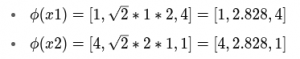
print("φ(x1):", phi_x1)
print("φ(x2):", phi_x2)
print("Dot product in transformed space:", explicit_dot)
print("Kernel function result:", kernel_dot)
Output You Should See
φ(x1): [1. 2.82842712 4. ]
φ(x2): [4. 2.82842712 1. ]
Dot product in transformed space: 16.0
Kernel function result: 16.0
Interpretation
- We explicitly transformed x1 and x2 using ϕ
- We then calculated their dot product: 16.0
- We used the kernel trick to get the same result without the transformation: 16.0
This shows how kernels bypass the expensive computation of high-dimensional features while achieving the same result.
Why Different Kernels?
Because data relationships differ:
- Some are linear (straight-line)
- Some are curvy but smooth
- Some have sudden changes or clusters
- Some need periodic understanding (like time-series or sound)
So, the kernel function should match the pattern of our problem.
Common Kernel Functions — and When to Use Them
| Kernel | Formula | Use Case | Why Use It |
|---|---|---|---|
| Linear | K(x, x′) = xTx′ | Text classification, linear regression, high-dimensional sparse data | Simple, fast, works well when features are already meaningful |
| Polynomial | K(x, x′) = (xTx′ + c)d | Complex interactions (e.g., XOR logic) | Captures feature interactions, nonlinear behavior |
| RBF (Gaussian) | 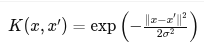 |
Smooth nonlinear functions (regression/classification), image data | Infinite-dimensional, captures locality (similar inputs give similar outputs) |
| Sigmoid | K(x, x′) = tanh(αxTx′ + c) | Neural network-style problems | Inspired by activation functions in neural nets |
| Periodic | 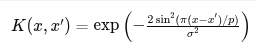
|
Time series with repeating patterns (weather, seasons) | Captures repeating behavior |
| Custom | You define it! | Domain-specific knowledge | Tailored for DNA sequences, graphs, etc. |
Examples by Problem Type
| Problem Type | Best Kernel(s) | Why? |
|---|---|---|
| Stock Price Prediction | RBF / Periodic | Stock data is nonlinear, often seasonal or volatile |
| Text Classification (e.g., spam detection) | Linear | Sparse, high-dim data – linear kernel is fast & effective |
| Image Recognition | RBF / Polynomial | Need to capture localized features (edges, textures) |
| Voice/Speech Analysis | Periodic / RBF | Speech patterns repeat — need periodic + smooth transitions |
| Handwriting Digit Classification | RBF | Fine-grained variation in stroke shapes, needs smooth similarity |
| Biological Sequence Matching | String kernels / Custom | Need to compare patterns like “GCTA” vs “GTTA” using alignment logic |
How to Choose?
Here’s a rule-of-thumb process:
- Start with Linear: It’s fast, interpretable. If it fails → nonlinear.
- Try RBF: Great general-purpose kernel.
- Use Polynomial if our features are already engineered for interactions.
- Use Domain-Knowledge to pick (e.g., periodic kernel for seasonality).
- Cross-validation is our friend — test multiple kernels and compare performance.
Comparison Data
| x | RBF Kernel Prediction | Polynomial Kernel Prediction |
|---|---|---|
| 0.0 | 0.19373498590261296 | 0.9107058270501742 |
| 0.002004008016032064 | 0.20131810412152146 | 0.9091002689880323 |
| 0.004008016032064128 | 0.20897935310171012 | 0.907468010667257 |
| 0.0060120240480961915 | 0.2167171628945829 | 0.9058091700350044 |
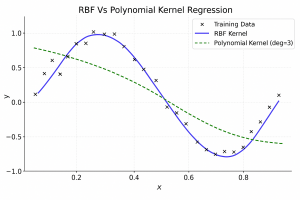
The chart above shows how two different kernels handle the same nonlinear dataset:
- RBF Kernel creates a smooth, flexible curve that closely follows the wavy sine-like pattern.
- Polynomial Kernel (degree 3) captures some curvature but is less flexible and smooth.
The table gives us exact prediction values from both models for comparison.This demonstrates how the choice of kernel changes the model’s behavior — and why it’s important to match the kernel to your problem type.
Python Script:
import numpy as np
import matplotlib.pyplot as plt
from sklearn.kernel_ridge import KernelRidge
import pandas as pd

# Step 1: Generate Sample Data (nonlinear sine wave + noise)
np.random.seed(0)
X = np.linspace(0, 1, 50).reshape(-1, 1)  # Features: 50 points from 0 to 1
y = np.sin(2 * np.pi * X).ravel() + np.random.normal(0, 0.1, X.shape[0])  # y = sin(2πx) + noise

# Step 2: Prepare test points for prediction
X_test = np.linspace(0, 1, 500).reshape(-1, 1)

# Step 3: RBF Kernel Regression
rbf_model = KernelRidge(kernel='rbf', alpha=0.1, gamma=25)
rbf_model.fit(X, y)
y_rbf = rbf_model.predict(X_test)

# Step 4: Polynomial Kernel Regression (degree 3)
poly_model = KernelRidge(kernel='polynomial', alpha=0.1, degree=3, coef0=1)
poly_model.fit(X, y)
y_poly = poly_model.predict(X_test)

# Step 5: Plot results
plt.figure(figsize=(12, 6))
plt.scatter(X, y, color='black', label='Training Data', alpha=0.6)
plt.plot(X_test, y_rbf, color='blue', label='RBF Kernel')
plt.plot(X_test, y_poly, color='green', linestyle='--', label='Polynomial Kernel (deg=3)')
plt.title("RBF vs Polynomial Kernel Regression")
plt.xlabel("x")
plt.ylabel("y")
plt.legend()
plt.grid(True)
plt.show()

# Step 6: Optional — Save comparison table
comparison_df = pd.DataFrame({
    "x": X_test.ravel(),
    "RBF Kernel Prediction": y_rbf,
    "Polynomial Kernel Prediction": y_poly
})
comparison_df.to_csv("kernel_comparison_output.csv", index=False)
Sample Data Snapshot
This is the X and y generated:
X (input): [0.0, 0.0204, …, 0.98, 1.0] — 50 points
y (output): sin(2πx) + noise — non-linear with random variation
Dependencies
Install these if needed:
pip install numpy matplotlib scikit-learn pandas
Kernel in Regression – Basic Math Concepts