Gradient Descent example with Simple Python
SIMPLE PYTHON EXAMPLE (WITHOUT ANY LIBRARY)
Let’s say we have a simple linear neuron: y = w * x
We want to minimize the squared error between prediction and actual y.
# Gradient Descent to learn y = 2x

# Step 1: Sample data
x_data = [1, 2, 3, 4]
y_data = [2, 4, 6, 8]  # Perfect: y = 2 * x

# Step 2: Initialize weight
w = 0.0

# Step 3: Learning rate
lr = 0.01

# Step 4: Training loop
for epoch in range(50):
    total_loss = 0
    dw = 0  # gradient accumulator
    for x, y_true in zip(x_data, y_data):
        y_pred = w * x
        loss = (y_pred - y_true) ** 2
        total_loss += loss
        dw += 2 * x * (y_pred - y_true)  # derivative of loss w.r.t w

    w -= lr * dw / len(x_data)  # average gradient update
    print(f"Epoch {epoch+1}: w = {w:.4f}, loss = {total_loss:.4f}")
EXPLANATION
- We simulate a tiny neural net with 1 weight w.
- Goal: Make w close to 2 because y = 2x.
- Each iteration (epoch), we calculate the gradient (dw) and update w.
- The loss (squared error) gets smaller — meaning we’re learning.
HOW THE LOSS REDUCES (CONCEPTUALLY)
| Epoch | Weight (w) | Loss |
|---|---|---|
| 1 | 0.56 | 120.00 |
| 5 | 1.85 | 4.00 |
| 10 | 1.98 | 0.15 |
| 50 | ~2.00 | ~0.00 |
FINAL RECAP
- Why: To reduce prediction error
- What: Iteratively update weights using gradients
- How: Move weights opposite to the gradient of the loss
- Where: Used in every neural network training process
A graph showing loss reduction visually:
Conceptual Loss Curve
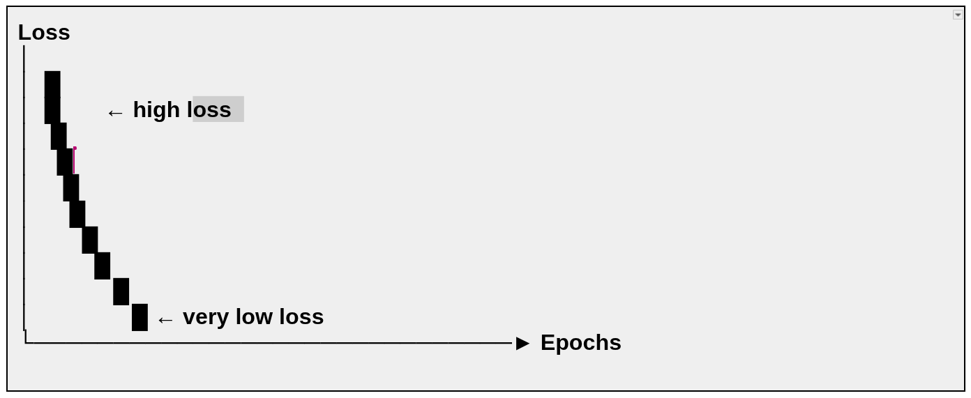
Y-axis: Total loss (squared error)
X-axis: Epoch number
As training progresses, the weight w gets closer to 2, and the error decreases.
Gradient Descent in Neural Network – Basic Math Concepts