Feedback Layer example with Simple Python
1. We’ll build:
- 1 input → 1 neuron → 1 output
- Our goal: learn the correct output using feedback (error correction)
- We’ll update the weight using a basic learning rule
Example: Learn to output 1 when input is 2
Learning Rule:
weight = weight + learning_rate * error * input
Python Code: Feedback Loop without any libraries
# Input and expected output
x = 2                 # input
y_true = 1            # target output

# Initial weight (bad guess)
weight = 0.1

# Learning rate (how fast we learn)
learning_rate = 0.01

# Track loss for each epoch
losses = []

# Training loop for 50 epochs
for epoch in range(50):
    # Step 1: Forward pass (guess)
    y_pred = x * weight

    # Step 2: Calculate error (feedback)
    error = y_true - y_pred
    loss = error ** 2  # simple squared error

    # Step 3: Adjust weight using feedback
    weight = weight + learning_rate * error * x

    # Step 4: Track progress
    losses.append(loss)

    # Print progress
    print(f"Epoch {epoch+1}: Prediction = {round(y_pred, 4)}, Error = {round(error, 4)}, Weight = {round(weight, 4)}, Loss = {round(loss, 4)}")

# Final result
print("\nFinal Weight:", round(weight, 4))
Output:
Epoch 1: Prediction = 0.2, Error = 0.8, Weight = 0.116, Loss = 0.64
Epoch 2: Prediction = 0.232, Error = 0.768, Weight = 0.1314, Loss = 0.5898
….
….
….
Epoch 49: Prediction = 0.8873, Error = 0.1127, Weight = 0.4459, Loss = 0.0127
Epoch 50: Prediction = 0.8918, Error = 0.1082, Weight = 0.448, Loss = 0.0117Final Weight: 0.448
What You’ll Observe:
- The prediction gets closer to 1 (our target)
- The error becomes smaller
- The weight adjusts itself using feedback
- Loss reduces over epochs
ASCII Visualization of Loss Decrease
We can visualize it manually like this:
# Draw loss reduction chart
print("\nLoss reduction (ASCII chart):")
for i, loss in enumerate(losses):
    bar = "#" * int(50 * (loss / max(losses)))  # normalized bar
    print(f"Epoch {i+1:02d}: {bar} ({round(loss, 4)})")
In Simple Words:
The network makes a guess, receives feedback, adjusts itself, and repeats — just like a person practicing and improving each time.
2. The logic behind adjusting weights after the output layer result.
The Big Idea (in simple terms):
The network makes a prediction. We compare it to the correct answer. If it’s wrong, we change the weights so the next prediction is less wrong.
Why do we adjust the weights?
Think of weights like knobs on a machine:
- They control how much influence each input has.
- If the output is too high or too low, we “tune the knobs” to fix it — that’s what adjusting the weights does.
Step-by-step Explanation
Let’s say:
- Input: x
- Current weight: w
- Prediction: y_pred = x * w
- Correct answer: y_true
- Error: error = y_true – y_pred
- Learning rate: lr (small number to control how big the weight change is)
Update Rule (Gradient Descent for 1 neuron):
w = w + (lr * error * x)
What does each part mean?
| Part | Meaning |
|---|---|
| error | How wrong was the prediction? |
| x | How much the input contributed to the wrong prediction |
| lr | Controls how big the update should be |
| w + … | We adjust the weight to improve the next prediction |
Intuitive Logic:
- If the error is positive, the prediction was too low → increase the weight.
- If the error is negative, the prediction was too high → decrease the weight.
- If the error is zero, prediction is correct → no change needed.
Real-Life Analogy:
Imagine adjusting a recipe for soup:
- We taste it and it’s too salty (wrong output).
- We reduce the salt next time (adjust the “weight” of the salt).
- Keep repeating until it tastes just right (low error).
Looping this = Learning!
Every time we:
- Predict →
- Compare with actual result →
- Adjust the weights →
- Repeat…
…our model learns better behavior.
Weight Adjustment Logic Flow (Markdown Diagram)
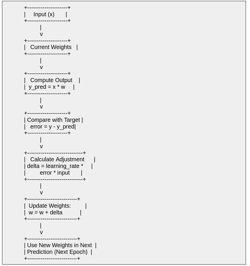
Summary:
- Compute output
- Check error
- Adjust weights using error
- Use updated weights next time
Feedback Layer relevancy of Neural Network – Visual Roadmap