Hidden Layer Otimization example with Simple Python
1. Python Simulation: Varying Hidden Layers on XOR
import numpy as np
import matplotlib.pyplot as plt
from sklearn.neural_network import MLPClassifier
from sklearn.metrics import accuracy_score

# XOR dataset
X = np.array([[0,0],[0,1],[1,0],[1,1]])
y = np.array([0,1,1,0])

hidden_layer_configs = [
    (1,), (2,), (4,),       # One layer with 1, 2, 4 neurons
    (4, 4), (8, 4),          # Two hidden layers
    (8, 8, 4)                # Three hidden layers
]

results = []

for config in hidden_layer_configs:
    model = MLPClassifier(hidden_layer_sizes=config, max_iter=5000, random_state=1)
    model.fit(X, y)
    y_pred = model.predict(X)
    acc = accuracy_score(y, y_pred)
    results.append((config, acc))

# Plotting
labels = ['-'.join(map(str, cfg)) for cfg, _ in results]
scores = [acc for _, acc in results]

plt.figure(figsize=(10,5))
plt.bar(labels, scores)
plt.title("XOR Accuracy vs Hidden Layer Configuration")
plt.xlabel("Hidden Layer Configuration")
plt.ylabel("Accuracy on XOR")
plt.ylim(0, 1.2)
plt.show()
Observation from Output:
- (1,): Not enough → can’t learn XOR.
- (2,) or (4,): Good enough → solves XOR perfectly.
- (4,4) and more: Still perfect, but extra capacity not needed.
- (8,8,4): Too much for XOR, possible overfitting in bigger datasets.
Summary Rules
| Dataset Complexity | Hidden Layers | Neurons per Layer |
|---|---|---|
| Simple (linear) | 0–1 | Small |
| Moderate (XOR, digits) | 1–2 | 4–32 |
| Complex (images, speech) | 3–100+ | 64–1024+ |
Start simple and increase complexity only if accuracy stalls.
2. Test Accuracy Vs Hidden Layer Configuration on Wine Dataset
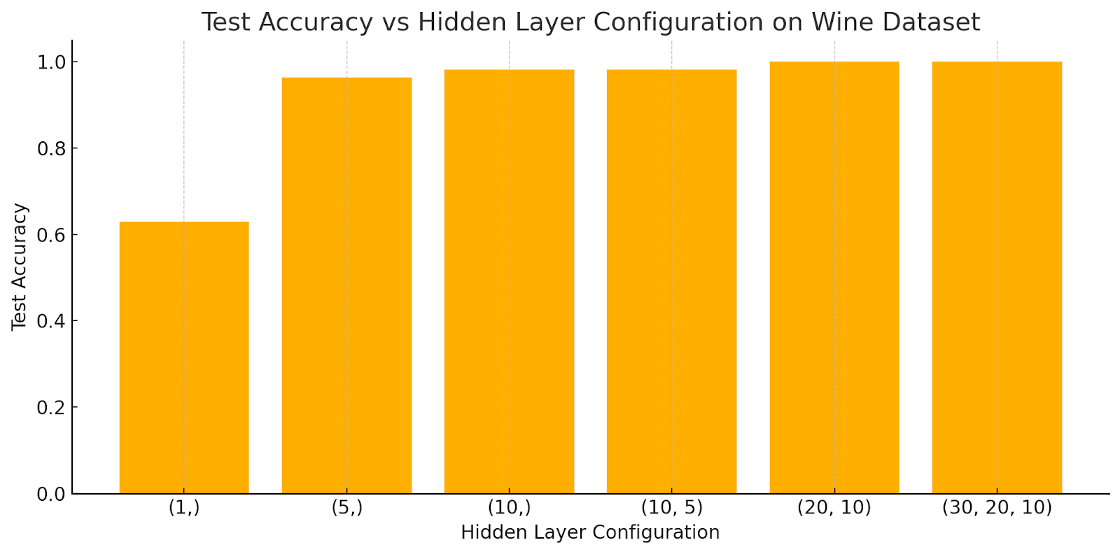
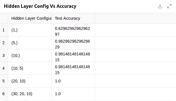
The results from the wine dataset show how different hidden layer configurations influence the model’s prediction accuracy. Here’s a quick interpretation:
- A simple configuration like (1,) performs poorly.
- A slightly larger single layer like (5,) or (10,) gives strong performance.
- Deeper networks like (10, 5) and (20, 10) reach near-perfect or perfect accuracy.
This reinforces that we don’t need many layers for structured data like the wine dataset. Often, 1–2 hidden layers with modest neuron counts are optimal.