Pattern Detector Design Approach with Simple Python
Goal:
From an image of a window, detect its:
- Edges (borders of window panes)
- Corners (where vertical and horizontal lines meet)
Step-by-Step Flow: From Image to Information Extraction
Step 1: Input – Represent the Window Image
Think of a simplified grayscale image (no colors), represented as a 2D matrix:
[
[100, 100, 100, 100, 100], ← wall
[100, 20, 20, 20, 100], ← window frame
[100, 20, 255, 20, 100], ← window glass center bright
[100, 20, 20, 20, 100], ← window frame
[100, 100, 100, 100, 100] ← wall
]
Observation:
- Edges (change from 100 → 20 or 20 → 255)
- Corners (where horizontal and vertical changes meet)
Step 2: Choose Pattern Detectors (Kernels)
We use known edge and corner detection kernels.
Horizontal Edge Detector (Sobel):
[[-1, -2, -1],
[ 0, 0, 0],
[ 1, 2, 1]]
Vertical Edge Detector (Sobel):
[[-1, 0, 1],
[-2, 0, 2],
[-1, 0, 1]]
Corner Detector (Harris-like idea):
This combines horizontal + vertical edges or uses something like:
[[-1, -1, -1],
[-1, 8, -1],
[-1, -1, -1]]
Step 3: Apply the Convolution Operation
Slide the kernel (3×3) over the image matrix. For each 3×3 patch:
- Multiply element-wise.
- Sum the result.
- The result goes in the corresponding cell of output matrix.
We get a new matrix (called feature map), showing how strong the edge/corner is at each point.
Step 4: Output Feature Maps
Each kernel will produce a new image-like matrix:
- Horizontal edge map: Bright lines = horizontal edges
- Vertical edge map: Bright lines = vertical edges
- Corner map: Bright points = corners
Step 5: Combine and Threshold
We now combine outputs or threshold them:
- Any value > threshold → “Edge exists”.
- Corners exist where both vertical + horizontal strengths are high.
Step 6: Information Extraction
Now we can say:
- “Window has 4 corners at positions (x, y)…”
- “Edges found along frame lines…”
- Use this in downstream tasks like:
- Geometry extraction
- Shape recognition
- 3D structure estimation
Output Visualization (Example)
Let’s say after convolution:
- Edge map shows bright outline around the window frame
- Corner map shows white dots at 4 corners of window panes
This is the information extracted.
What Did We Learn?
| Concept | Explanation |
|---|---|
| Image | 2D matrix |
| Edge | Sharp intensity change (detected by gradient) |
| Kernel | Pattern detector matrix |
| Convolution | Sliding the kernel and generating feature maps |
| Feature Map | Output showing where features (edges/corners) exist |
| Information | Edge positions, corner coordinates |
Window Image Matrix (Simplified Input)
Let’s take this 5×5 grayscale image where:
- 100 = wall
- 20 = window frame (darker)
- 255 = bright glass center
Step 1: Original Image Matrix
| 100 | 100 | 100 | 100 | 100 |
| 100 | 20 | 20 | 20 | 100 |
| 100 | 20 | 255 | 20 | 100 |
| 100 | 20 | 20 | 20 | 100 |
| 100 | 100 | 100 | 100 | 100 |
Step 2: Choose Pattern Detector (Kernels)
A. Vertical Edge Kernel (Sobel)
| -1 | 0 | 1 |
| -2 | 0 | 2 |
| -1 | 0 | 1 |
B. Horizontal Edge Kernel (Sobel)
| -1 | -2 | -1 |
| 0 | 0 | 0 |
| 1 | 2 | 1 |
C. Corner Detector (Laplacian)
| -1 | -1 | -1 |
| -1 | 8 | -1 |
| -1 | -1 | -1 |
Step 3: Apply Convolution at Center (3×3)
Take center region (from rows 2–4, cols 2–4):
| 20 | 20 | 20 |
| 20 | 255 | 20 |
| 20 | 20 | 20 |
Vertical Edge Output:
Apply element-wise multiplication with vertical kernel:
(-1×20) + (0×20) + (1×20) +
(-2×20) + (0×255) + (2×20) +
(-1×20) + (0×20) + (1×20)
= (-20 + 0 + 20) + (-40 + 0 + 40) + (-20 + 0 + 20) = 0
No vertical edge at center.
Horizontal Edge Output:
(-1×20) + (-2×20) + (-1×20) +
( 0×20) + ( 0×255) + ( 0×20) +
( 1×20) + ( 2×20) + ( 1×20)
= (-20 -40 -20) + (0) + (20 + 40 + 20) = -80 + 80 = 0
No horizontal edge at center either.
Corner Detector Output:
(-1×20) + (-1×20) + (-1×20) +
(-1×20) + (8×255) + (-1×20) +
(-1×20) + (-1×20) + (-1×20)
= -20×8 + 2040 = -160 + 2040 = **1880**
Strong corner detected!
Step 4: Feature Map Output Table
| Position (Center of 3×3) | Vertical Edge | Horizontal Edge | Corner Score |
|---|---|---|---|
| (2,2) | 0 | 0 | 1880 |
| (2,3) | … | … | … |
| (3,2) | … | … | … |
Repeat for all center positions)
Step 5: Threshold & Final Result
After calculating values across image:
Any corner score > 1000 → mark as corner
Any edge score > threshold → mark as edge
Final Information Extracted
| Feature Type | Location (Row, Col) | Description |
|---|---|---|
| Corner | (2,2) | Central window cross-point |
| Edge | (1,2), (2,1), etc. | Detected from respective kernel outputs |
| Shape | Likely rectangle | Inferred from edge layout |
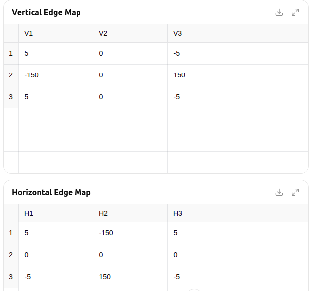
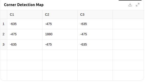
Here are the simulation results from the Python program showing the feature maps extracted using convolution:
- Vertical Edge Map – highlights vertical changes
- Horizontal Edge Map – highlights horizontal changes
- Corner Detection Map – highlights sharp changes (corners)
The center value 1880 in the Corner Detection Map confirms a strong corner detected at the center of the window. We can interpret the rest of the values similarly to locate edges and corners in the image.
Here is the complete Python script that we can run locally to simulate edge and corner detection on a simplified 5×5 grayscale window image using convolution:
import numpy as np
import pandas as pd
from scipy.signal import convolve2d
import matplotlib.pyplot as plt
import seaborn as sns

# Step 1: Define the 5x5 grayscale image (simulated window)
image = np.array([
    [100, 100, 100, 100, 100],
    [100,  20,  20,  20, 100],
    [100,  20, 255,  20, 100],
    [100,  20,  20,  20, 100],
    [100, 100, 100, 100, 100]
])

# Step 2: Define convolution kernels
vertical_kernel = np.array([
    [-1, 0, 1],
    [-2, 0, 2],
    [-1, 0, 1]
])

horizontal_kernel = np.array([
    [-1, -2, -1],
    [ 0,  0,  0],
    [ 1,  2,  1]
])

corner_kernel = np.array([
    [-1, -1, -1],
    [-1,  8, -1],
    [-1, -1, -1]
])

# Step 3: Apply convolution (valid mode = center-only scan)
vertical_edges = convolve2d(image, vertical_kernel, mode='valid')
horizontal_edges = convolve2d(image, horizontal_kernel, mode='valid')
corner_response = convolve2d(image, corner_kernel, mode='valid')

# Step 4: Display output as tables
print("Vertical Edge Map:\n", pd.DataFrame(vertical_edges))
print("\nHorizontal Edge Map:\n", pd.DataFrame(horizontal_edges))
print("\nCorner Detection Map:\n", pd.DataFrame(corner_response))

# Optional: visualize heatmaps
plt.figure(figsize=(12, 4))
titles = ["Vertical Edges", "Horizontal Edges", "Corner Detection"]
data_maps = [vertical_edges, horizontal_edges, corner_response]

for i, data in enumerate(data_maps):
    plt.subplot(1, 3, i + 1)
    sns.heatmap(data, annot=True, fmt="d", cmap="coolwarm", cbar=False)
    plt.title(titles[i])
plt.tight_layout()
plt.show()
How It Works:
- Uses scipy.signal.convolve2d for convolution
- Applies three filters (vertical, horizontal, corner)
- Prints the result as tables
- Plots the output using heatmaps for easy understanding