First and Second Derivatives in Neural Networks
1. First-Order Derivative
- Refers to the gradient.
- In neural networks, it’s used to compute how much the loss function changes with respect to the weights.
- It’s the backbone of gradient descent.
In simple terms: It tells us the slope — how to adjust the weights to reduce error.
2. Second-Order Derivative
- Refers to the Hessian or curvature.
- It helps to understand how the gradient itself is changing.
- It is used in Newton’s method, optimization refinement, and to detect saddle points or curvature.
In simple terms: It tells us how “bendy” or steep the slope is — whether we’re on a hill, a valley, or a flat saddle.
3. Role in Neural Networks
| Derivative | Role | Where It Appears |
|---|---|---|
| First-order | Guide weight updates | In backpropagation during training |
| Second-order | Refines optimization, handles curvature | In advanced optimizers like Newton’s method or L-BFGS |
4. Mathematical Foundation
First-Order: Gradient
For a loss function L(w) with respect to weights w:
∂L / ∂w
Used directly in:
w=w−η⋅∂L / ∂w
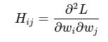
Second-Order: Hessian
Hessian matrix H is:
H=∂^2L / ∂w^2
It’s a square matrix of second-order partial derivatives:
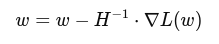
Used in:
5. Global Minimum
- The lowest point in the entire loss landscape.
- It’s where the loss function attains its absolute minimum.
6. Local Minimum
- A point where the loss is lower than all nearby points, but not necessarily the lowest overall.
- We can get “stuck” here during training.
7. Saddle Point
- Not a minimum at all; it’s a point where the gradient is zero, but the curvature is positive in one direction and negative in another.
8. Resemblance to Derivatives
| Feature | Derivative Connection |
|---|---|
| Local/Global Minimum | It occurs where the first-order derivative = 0 (i.e., flat slope) |
| Type of Stationary Point | Determined by the second-order derivative |
| Saddle Point Detection | First derivative = 0, but second-order derivative < 0 in some direction |
9. Visual Analogy
Imagine a 2D loss function (like a bumpy valley):
- Gradient (1st Derivative) tells the direction and steepness: we follow the negative gradient to descend.
- When the gradient becomes zero, we’re at a stationary point. This could be:
- A local minimum (valley)
- A saddle point (flat but not lowest)
- A maximum (peak)
The second-order derivative (curvature) helps distinguish between these:
| Case | 1st Derivative | 2nd Derivative |
|---|---|---|
| df/dx = 0, d²f/dx² > 0 | Flat slope | Upwards curve — Likely a minimum |
| df/dx = 0, d²f/dx² < 0 | Flat slope | Downward curve — Likely a maximum |
| df/dx = 0, d²f/dx² ≈ 0 or mixed signs | Flat slope | No clear curve — Could be a saddle point |
10. Neural Network Example
Suppose we’re training a neural network and our loss function looks like this (conceptually):
Loss
^
| *
| * *
| * * ← Local minima (bad but looks okay)
| * *
| * *
|____________________> Weights
*
* *
* * ← Global minimum
- Our optimizer (like SGD) follows the gradient (1st derivative).
- If we hit a flat spot (gradient ≈ 0), it stops moving.
- Without knowing the second derivative, we can’t tell if that flat spot is:
- A real minimum
- Or a saddle point that you should escape
Some optimizers like Adam and RMSProp help escape local minima or saddle points by including momentum or adaptive learning rates, but they don’t directly use the second derivative.
11. Summary Table
| Concept | First Derivative | Second Derivative | Meaning |
|---|---|---|---|
| Global Minima | Zero slope | Positive definite Hessian | Best solution |
| Local Minima | Zero slope | Positive but not global | Acceptable, not optimal |
| Saddle Point | Zero slope | Mixed or zero curvature | Needs an escape strategy |
12. What is a Saddle Point?
A saddle point is a point on the loss surface where:
- The gradient (first derivative) is zero — so it looks like a minimum or maximum in some directions.
- But it is not a minimum overall — because the surface curves up in one direction and down in another.
Real-Life Analogy
Imagine sitting on a horse saddle:
- Along the length of the horse (front to back), the saddle curves upwards → like a hill (maximum).
- Along the width (side to side), it curves downwards → like a valley (minimum).
So from one view, we’re at a peak, and from another, we’re in a dip.
Mathematical Description
In a function f(x,y), a saddle point occurs when:
- ∇f=0 → first-order derivative is zero
- The Hessian matrix (second-order derivative) has mixed signs:
- One direction has positive curvature (like a bowl).
- Another has negative curvature (like a hill).
Example:
f(x,y)=x^2−y^2
At point (0,0):
- ∂f / ∂x=2x=0
- ∂f / ∂y=−2y=0
- But:
- Along the x-axis → f=x^2 → curve upward (minimum)
- Along the y-axis → f=−y^2 → curve downward (maximum)
- Most critical points are saddle points, not minima.
- Gradient descent slows down around them because the gradient is close to zero, and it gets “stuck”.
- Escaping them can be hard without help (e.g., random noise, momentum).
Hence, (0,0) is a saddle point.
Why Saddle Points Are a Problem in Neural Networks
In high-dimensional neural networks, saddle points are everywhere.
Optimizer Behavior at Saddle Points
| Optimizer | Behavior at Saddle Point |
|---|---|
| SGD | May stall (flat gradient) |
| Momentum | May pass through due to inertia |
| Adam | Uses adaptive steps, better at escaping |
| Newton’s Method | Can wrongly assume it’s a minimum and converge there (if Hessian is not handled well) |
First and Second Derivatives in Neural Networks – First and Second Derivatives Example with Simple Python