Prediction Error example with Simple Python
1. Simple Python Simulation (Without Libraries):
# Simple single-layer neural network prediction and error calculation

# True value (actual output)
y_true = 10

# Dummy weight and input
w = 0.8  # weight
x = 12   # input

# Bias
b = 2

# Prediction from the model
y_pred = w * x + b

# Error
error = y_true - y_pred

# Output
print("Predicted:", y_pred)
print("Actual:", y_true)
print("Prediction Error:", error)
Output:
Predicted: 11.6
Actual: 10
Prediction Error: -1.6
Significance of Error Over Time (During Training)
- Initially, prediction error is high.
- As we train the model (by adjusting weights and biases), the error should reduce.
- The error is used to compute the loss, and the loss is minimized using optimization algorithms.
Impact on Prediction:
- High error → model is not learning well → poor predictions.
- Reducing error over epochs → model is learning → better predictions.
- If error stops decreasing or increases again → possibly overfitting or underfitting.
2. Simple Neural Network Example (1 input → 1 output)
Goal:
Learn a function that predicts y = 2 * x + 1
Code with Backpropagation (Pure Python):
# Simple one neuron network with 1 weight, 1 bias, and backpropagation

# Training data
x = 2     # input
y_true = 5  # actual output (because 2*2 + 1 = 5)

# Initial parameters (random guesses)
w = 0.5   # weight
b = 0.0   # bias

# Learning rate (controls how much we adjust weights)
lr = 0.1

# Train for a few epochs
for epoch in range(10):
    # ---- Forward pass ----
    y_pred = w * x + b  # predicted output
    error = y_true - y_pred  # prediction error
    loss = error ** 2  # squared error

    # ---- Backpropagation (gradient calculation) ----
    # dL/dw = -2 * x * (y - y_pred)
    # dL/db = -2 * (y - y_pred)
    dL_dw = -2 * x * error
    dL_db = -2 * error

    # ---- Update weights and bias ----
    w = w - lr * dL_dw
    b = b - lr * dL_db

    # ---- Print progress ----
    print(f"Epoch {epoch+1}: y_pred={y_pred:.4f}, loss={loss:.4f}, w={w:.4f}, b={b:.4f}")
Explanation of What’s Happening:
- Forward pass:
Predict output using y_pred = w * x + b - Calculate error:
error = y_true – y_pred - Loss (Squared Error):
loss = error^2 – we want this to reduce over time - Backpropagation (derivatives of loss w.r.t. w and b):
These gradients tell us how much each parameter is responsible for the error - Weight update rule:
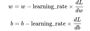
- Repeat for multiple epochs
Sample Output:
Epoch 1: y_pred=1.0000, loss=16.0000, w=1.3000, b=0.8000
Epoch 2: y_pred=3.4000, loss=2.5600, w=1.7800, b=1.2800
Epoch 3: y_pred=4.8400, loss=0.0256, w=1.9560, b=1.4560
…
Notice how:
- The loss decreases each epoch
- The weights and bias adjust closer to the correct values (w → 2, b → 1)
Prediction Error in Neural Network – Basic Math Concepts