Matplotlib Primer
Matplotlib Primer for AI and Deep Learning
Beginner Syntax
import matplotlib.pyplot as plt

# Line plot
x = [1, 2, 3, 4, 5]
y = [0.9, 0.7, 0.4, 0.3, 0.2]
plt.plot(x, y)
plt.title("Loss over Epochs")
plt.xlabel("Epoch")
plt.ylabel("Loss")
plt.grid(True)
plt.show()
    # Bar chart
features = ['A', 'B', 'C']
scores = [0.2, 0.5, 0.3]
plt.bar(features, scores)
plt.title("Feature Importance")
plt.xlabel("Features")
plt.ylabel("Score")
plt.show()
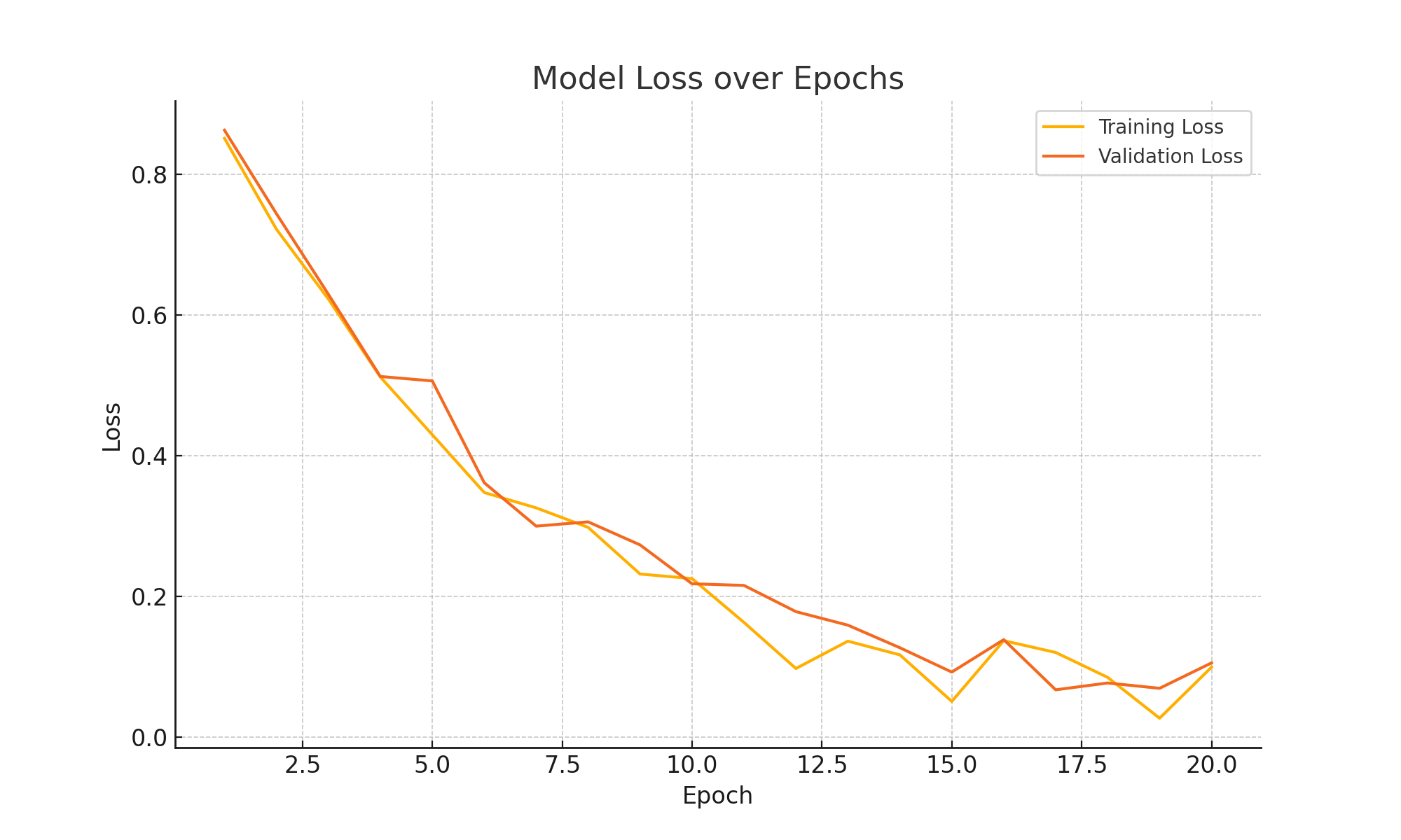
Loss Curve Visualization
import numpy as np
epochs = np.arange(1, 21)
train_loss = np.exp(-0.2 * epochs) + 0.1 * np.random.rand(20)
val_loss = np.exp(-0.18 * epochs) + 0.1 * np.random.rand(20)

plt.plot(epochs, train_loss, label='Training Loss')
plt.plot(epochs, val_loss, label='Validation Loss')
plt.xlabel('Epoch')
plt.ylabel('Loss')
plt.title('Model Loss over Epochs')
plt.legend()
plt.grid(True)
plt.show()
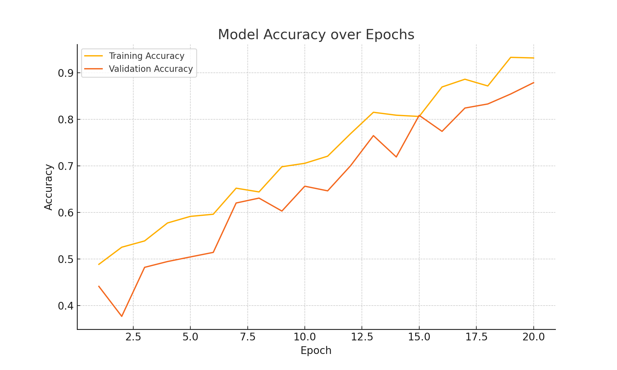
Accuracy Curve
train_acc = np.linspace(0.5, 0.95, 20) + 0.02 * np.random.randn(20)
val_acc = np.linspace(0.4, 0.9, 20) + 0.03 * np.random.randn(20)

plt.plot(epochs, train_acc, label='Training Accuracy')
plt.plot(epochs, val_acc, label='Validation Accuracy')
plt.xlabel('Epoch')
plt.ylabel('Accuracy')
plt.title('Model Accuracy over Epochs')
plt.legend()
plt.grid(True)
plt.show()
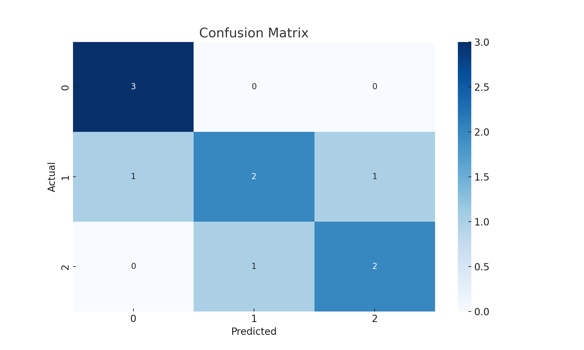
Confusion Matrix Heatmap
import seaborn as sns
from sklearn.metrics import confusion_matrix

y_true = [0, 1, 2, 2, 0, 1, 0, 2, 1, 1]
y_pred = [0, 2, 1, 2, 0, 0, 0, 2, 1, 1]
cm = confusion_matrix(y_true, y_pred)

sns.heatmap(cm, annot=True, fmt='d', cmap='Blues')
plt.xlabel("Predicted")
plt.ylabel("Actual")
plt.title("Confusion Matrix")
plt.show()
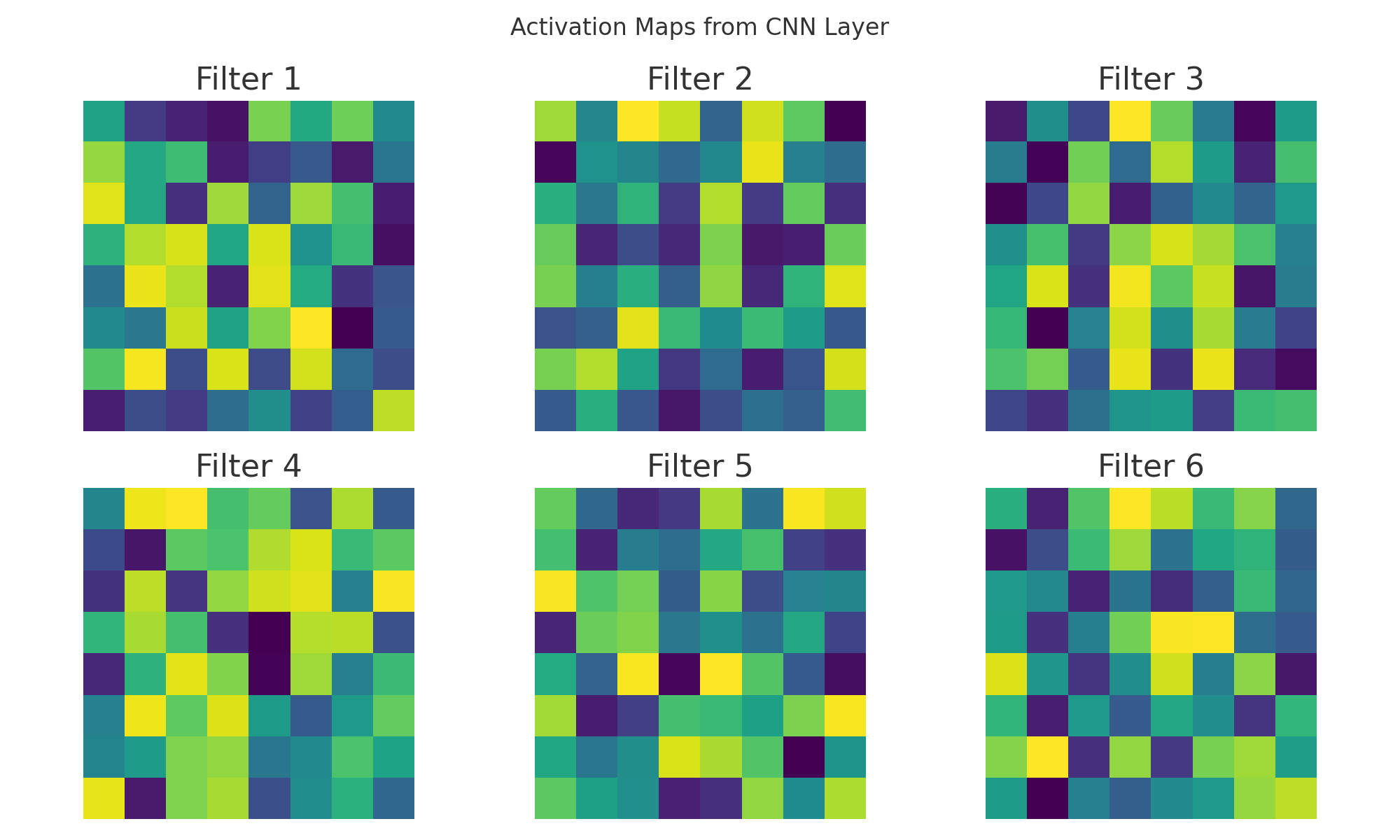
Activation Maps
activation_maps = np.random.rand(6, 8, 8)
fig, axes = plt.subplots(2, 3, figsize=(10, 6))
for i, ax in enumerate(axes.flat):
ax.imshow(activation_maps[i], cmap='viridis')
ax.set_title(f'Filter {i+1}')
ax.axis('off')
plt.suptitle('Activation Maps from CNN Layer')
plt.tight_layout()
plt.show()
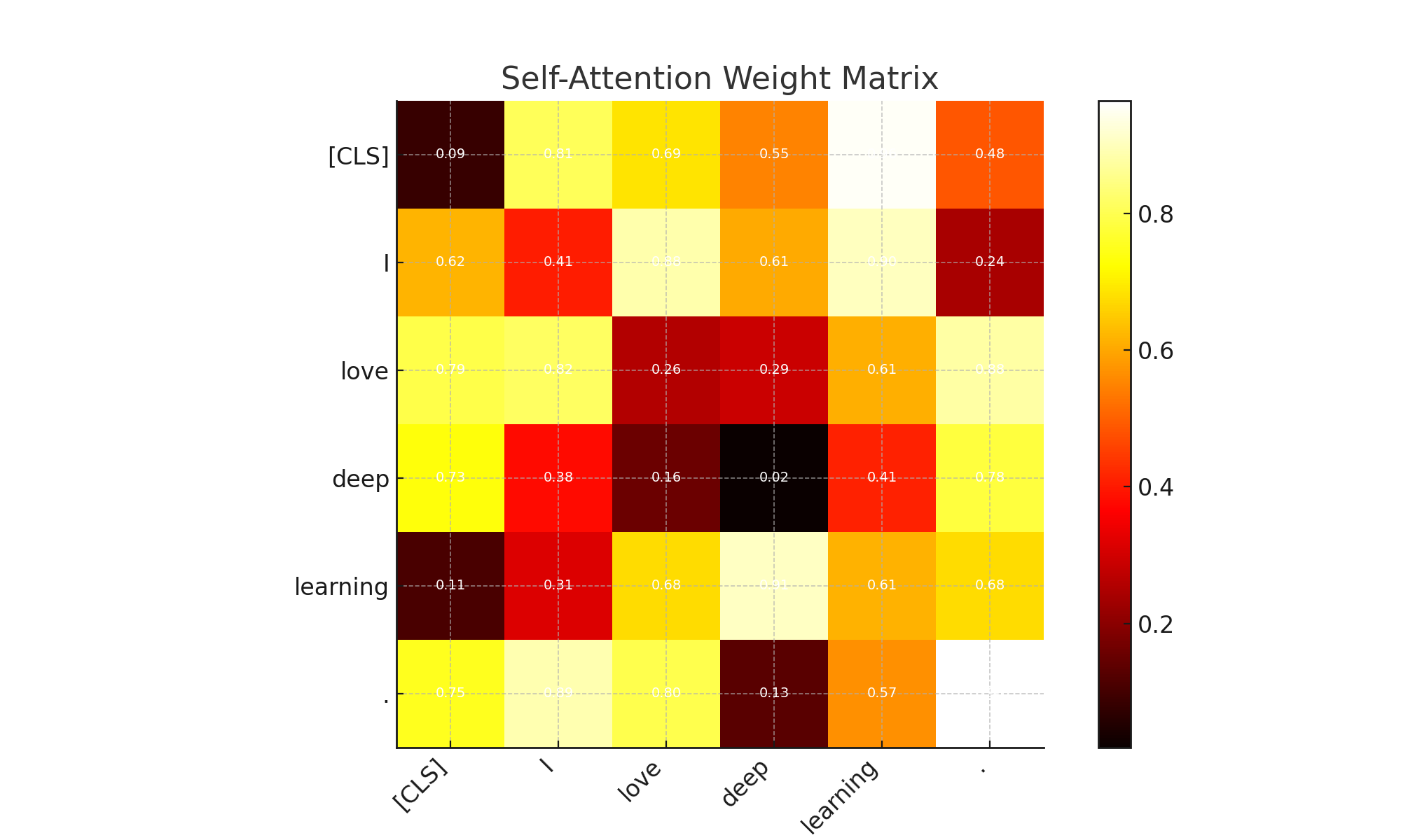
Attention Weights
tokens = ['[CLS]', 'I', 'love', 'deep', 'learning', '.']
attention_weights = np.random.rand(len(tokens), len(tokens))

fig, ax = plt.subplots()
im = ax.imshow(attention_weights, cmap='hot')

ax.set_xticks(np.arange(len(tokens)))
ax.set_yticks(np.arange(len(tokens)))
ax.set_xticklabels(tokens)
ax.set_yticklabels(tokens)
plt.setp(ax.get_xticklabels(), rotation=45, ha="right")

for i in range(len(tokens)):
for j in range(len(tokens)):
text = ax.text(j, i, f"{attention_weights[i, j]:.2f}", ha="center", va="center", color="w", fontsize=7)

ax.set_title("Self-Attention Weight Matrix")
plt.colorbar(im)
plt.show()
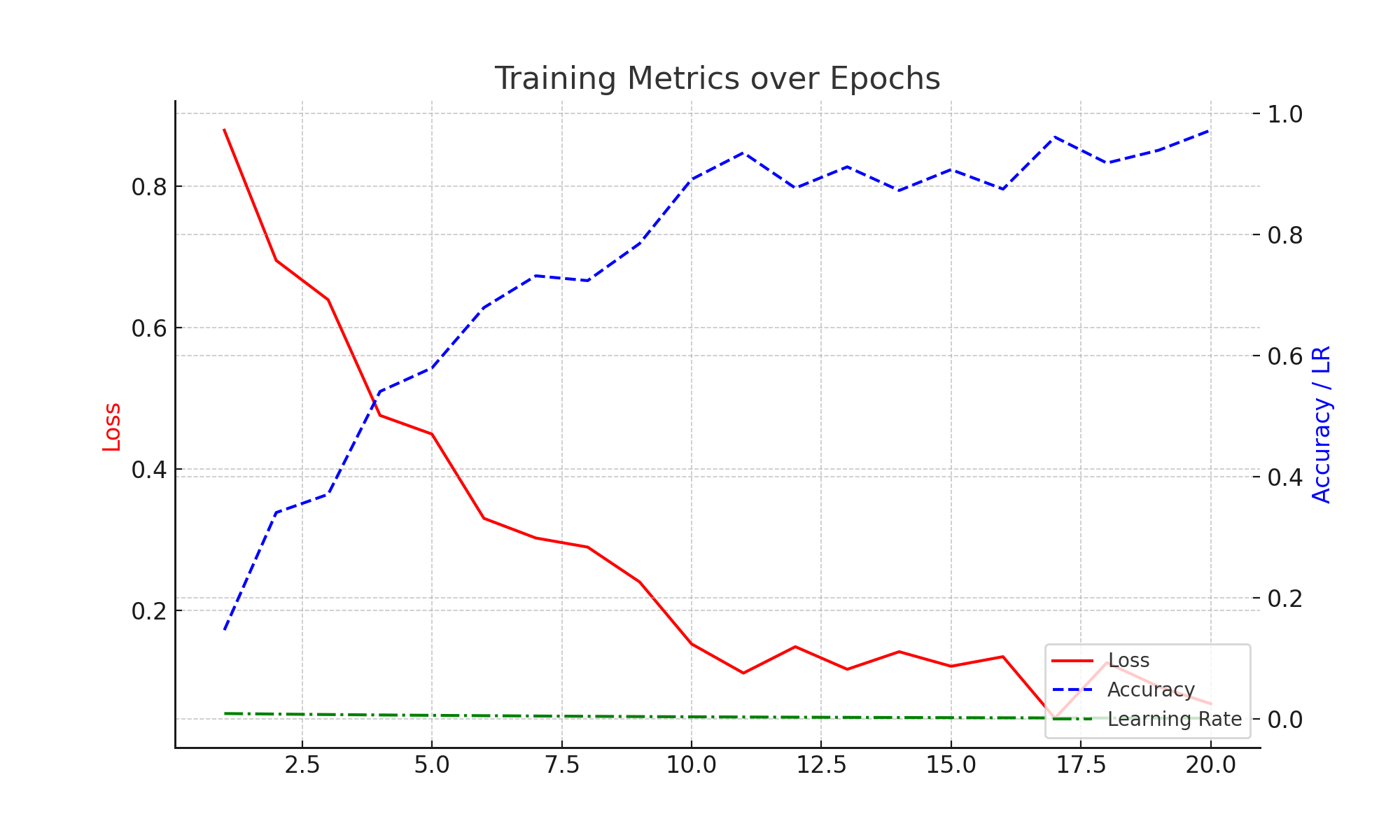
Training Logs (Loss, Accuracy, LR)
  loss = np.exp(-0.2 * epochs) + 0.1 * np.random.rand(20)
  accuracy = 1 - loss + 0.05 * np.random.rand(20)
  lr = 0.01 * np.exp(-0.1 * epochs)

  fig, ax1 = plt.subplots()
  ax1.plot(epochs, loss, 'r-', label='Loss')
  ax1.set_ylabel('Loss', color='red')

  ax2 = ax1.twinx()
  ax2.plot(epochs, accuracy, 'b--', label='Accuracy')
  ax2.plot(epochs, lr, 'g-.', label='Learning Rate')
  ax2.set_ylabel('Accuracy / LR', color='blue')

  lines, labels = ax1.get_legend_handles_labels()
  lines2, labels2 = ax2.get_legend_handles_labels()
  plt.legend(lines + lines2, labels + labels2, loc='lower right')

  plt.title('Training Metrics over Epochs')
  plt.grid(True)
  plt.show()
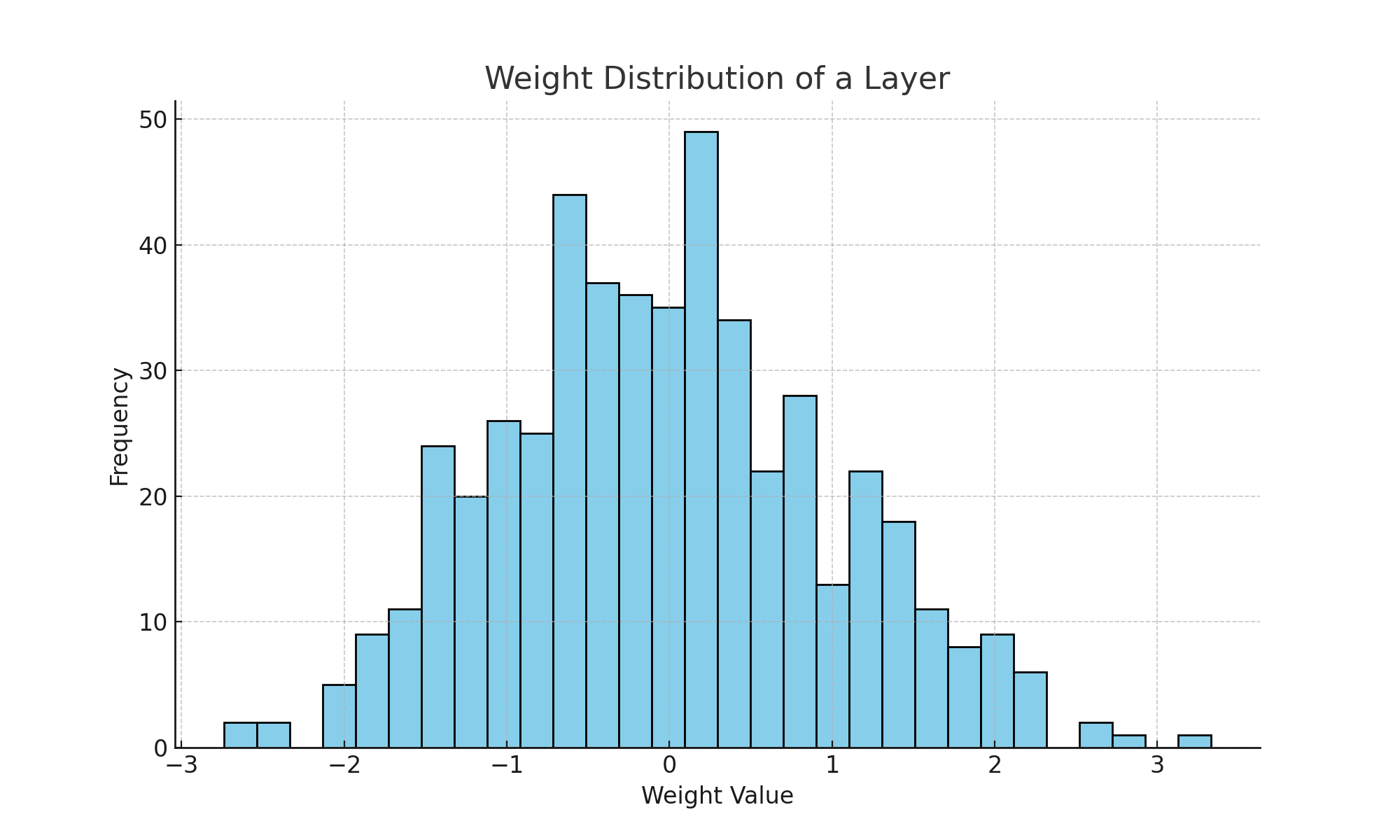
Weight Distribution
  layer_weights = np.random.normal(0, 1, 500)
  plt.hist(layer_weights, bins=30, color='skyblue', edgecolor='black')
  plt.title('Weight Distribution of a Layer')
  plt.xlabel('Weight Value')
  plt.ylabel('Frequency')
  plt.grid(True)
  plt.show()
Matplotlib Primer for AI & Deep Learning (with Code + Visuals)
Loss Curve
import numpy as np
epochs = np.arange(1, 21)
train_loss = np.exp(-0.2 * epochs) + 0.1 * np.random.rand(20)
val_loss = np.exp(-0.18 * epochs) + 0.1 * np.random.rand(20)
plt.plot(epochs, train_loss, label='Training Loss')
plt.plot(epochs, val_loss, label='Validation Loss')
plt.xlabel('Epoch')
plt.ylabel('Loss')
plt.title('Model Loss over Epochs')
plt.legend()
plt.grid(True)
plt.show()
Accuracy Curve
train_acc = np.linspace(0.5, 0.95, 20) + 0.02 * np.random.randn(20)
val_acc = np.linspace(0.4, 0.9, 20) + 0.03 * np.random.randn(20)
plt.plot(epochs, train_acc, label='Training Accuracy')
plt.plot(epochs, val_acc, label='Validation Accuracy')
plt.xlabel('Epoch')
plt.ylabel('Accuracy')
plt.title('Model Accuracy over Epochs')
plt.legend()
plt.grid(True)
plt.show()
Confusion Matrix
import seaborn as sns
from sklearn.metrics import confusion_matrix
y_true = [0, 1, 2, 2, 0, 1, 0, 2, 1, 1]
y_pred = [0, 2, 1, 2, 0, 0, 0, 2, 1, 1]
cm = confusion_matrix(y_true, y_pred)
sns.heatmap(cm, annot=True, fmt='d', cmap='Blues')
plt.xlabel("Predicted")
plt.ylabel("Actual")
plt.title("Confusion Matrix")
plt.show()
Activation Maps
activation_maps = np.random.rand(6, 8, 8)
fig, axes = plt.subplots(2, 3, figsize=(10, 6))
for i, ax in enumerate(axes.flat):
ax.imshow(activation_maps[i], cmap='viridis')
ax.set_title(f'Filter {i+1}')
ax.axis('off')
plt.suptitle('Activation Maps from CNN Layer')
plt.tight_layout()
plt.show()
Attention Weights
tokens = ['[CLS]', 'I', 'love', 'deep', 'learning', '.']
attention_weights = np.random.rand(len(tokens), len(tokens))
fig, ax = plt.subplots()
im = ax.imshow(attention_weights, cmap='hot')
ax.set_xticks(np.arange(len(tokens)))
ax.set_yticks(np.arange(len(tokens)))
ax.set_xticklabels(tokens)
ax.set_yticklabels(tokens)
plt.setp(ax.get_xticklabels(), rotation=45, ha="right")
for i in range(len(tokens)):
for j in range(len(tokens)):
ax.text(j, i, f"{attention_weights[i, j]:.2f}", ha="center", va="center", color="w", fontsize=7)
ax.set_title("Self-Attention Weight Matrix")
plt.colorbar(im)
plt.show()
Training Logs
loss = np.exp(-0.2 * epochs) + 0.1 * np.random.rand(20)
accuracy = 1 - loss + 0.05 * np.random.rand(20)
lr = 0.01 * np.exp(-0.1 * epochs)
fig, ax1 = plt.subplots()
ax1.plot(epochs, loss, 'r-', label='Loss')
ax1.set_ylabel('Loss', color='red')
ax2 = ax1.twinx()
ax2.plot(epochs, accuracy, 'b--', label='Accuracy')
ax2.plot(epochs, lr, 'g-.', label='Learning Rate')
ax2.set_ylabel('Accuracy / LR', color='blue')
lines, labels = ax1.get_legend_handles_labels()
lines2, labels2 = ax2.get_legend_handles_labels()
plt.legend(lines + lines2, labels + labels2, loc='lower right')
plt.title('Training Metrics over Epochs')
plt.grid(True)
plt.show()
Weight Distribution
layer_weights = np.random.normal(0, 1, 500)
plt.hist(layer_weights, bins=30, color='skyblue', edgecolor='black')
plt.title('Weight Distribution of a Layer')
plt.xlabel('Weight Value')
plt.ylabel('Frequency')
plt.grid(True)
plt.show()
Go to Core Learning